Ever wonder “How do I create a simple and easy to use PivotTable?”
PivotTables are tools you can use in a spreadsheet to quickly create interactive summary reports (tables) from raw data. Because they are interactive, PivotTables allow you to easily do any of the following:
- Summarize your data with various calculations including sum, average, maximum, and minimum.
- Display results across the page (horizontally) or down the page (vertically).
- Sort the results in ascending, descending, or a custom order.
- Filter the report to concentrate on what is important.
- “Drill down” to see the details behind a specific total.
As shown in the video above, you can follow these steps to create a PivotTable in Excel:
- Start Excel and create or open your file.
- Position the cursor in one cell, and only one cell, of the data.

Excel file with data
- From the ribbon choose Insert, Tables, PivotTable.

From the ribbon choose Insert, Tables, PivotTable
- In the create PivotTable dialog box make sure the table/range is referring to the correct table or range, and that the destination is a New Worksheet. Then click OK.

Create PivotTable dialog box
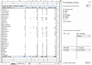
- Drag the fields from the PivotTable Field List to the desired location.

Drag PivotTable fields to the desired area
- Edit and format your completed PivotTable as desired.

Completed PivotTable
